
Look ma, I won the cup: A beaming Kapil Dev receiving the 1983 World Cup at Lord’s. Image source: 1.
66-1.
Almost every Indian sporting fan from an earlier era will probably instantly recognize these odds. For the uninitiated, these were the odds that the bookmakers were offering when Kapil Dev led the Indian team against the West Indies in their inaugural match of the 1983 World Cup.
66-1. Meaning, a 670 quid payout for a 10 quid punt (including the 10 from the initial bet). Dazzling odds, yes. But would anyone take a chance on the Indian team of the 1983 World Cup, even at those odds?
Let’s see what the Indian team had produced so far. Until the 1983 World Cup, India had won only 12 out of its 40 matches. In terms of Win-Loss ratio, it was ahead of only Sri Lanka, a team which had obtained test status only the previous year (Canada and East Africa had played only in the World cups). In the World cups, the team had done even worse—India had won only one match, that too against lowly East Africa. Coming into the tournament, the Indian team even lost a warm-up match against a team of farmers and salesmen. Now, looking at this evidence, would you fancy a bet?
It wasn’t that India didn’t produce good ODI results; just that they were rare. Earlier in March 1983, they had scored a morale boosting victory against the mighty West Indies in Berbice. They even managed to beat them in their opening match of the World Cup—so their result in Berbice was no fluke. They looked down and out of the World cup when they were struggling at 17 for 5 against Zimbabwe—having been crushed comprehensively by Australia and West Indies earlier—but for Kapil Dev’s once-in-a-lifetime innings. With England safely negotiated in the semifinals, the two-time champion team of West Indies would face them in the finals. Gulp. No chance, isn’t it? But how large was the scale of the challenge that was presented to them in the finals?
The one day international (ODI) in 1983 was vastly different from the matches that are played today’s age. Back then, it was played largely during the day, with a red ball, each innings lasted 60 overs, and hadn’t seen various iterations of fielding restrictions. Winning totals were much smaller and batsmen at the top of the order played the game as if it were an abridged version of a test match. Keeping this in mind, is there a way to mine the various statistics over the course of ODI history and come up with a way to measure the effectiveness of an ODI bowler?
As explored in earlier articles, the ODIs can be conveniently split into nine eras, with the last one ending on 31st December 2016. These eras contain at least one world tournament of significance, and have enough matches to observe trends.

Defining era: Each time period has at least 250 matches.
The game of cricket may be based on a contest between bat and ball, but there are some inherent differences between the roles played between batsmen and bowlers. For example, it is quite routine for all eleven players to get to bat in an ODI innings but very rare for more than seven bowlers to bowl in an ODI innings. Also, subsequent batsmen get a chance to bat only once a previous one is dismissed (unless injury plays a part), but bowlers can bowl any two or more non-successive overs in an innings provided their individual quota has not been exhausted.
The primary currency of a bowler in cricket is wickets. Compared to runs that can be scored by a batsman, they are relatively finite. For instance, the maximum tally that an ODI bowler can amass in an ODI innings is 10, but a batsman can in principle make 200 (or more) runs. Therefore, an approximate measure of equivalence between individual batting and bowling achievements has to be obtained before we proceed to dissect bowling statistics.

Frequency distribution of individual wicket hauls and run tallies in an ODI innings
Career statistics pages for bowlers often parade the five wicket haul as the bowling equivalent of a hundred. However, the frequency of occurrence a 5 wicket haul (~1%) is lesser compared to a score of 100 and above. That being the case, the quantum of the bowling benchmark has to be adjusted accordingly. ~42% of ODI innings end with a single digit score, which can be roughly equated to a zero wicket haul. Of course, sorting by magnitude has its own problems as a case can be made for a 2/13 haul or 34(13) being better than a 3/80 or 42(120), one of many other such discrepancies; but in the absence of other simple methods this can serve as a decent approximation to equate individual batting and bowling performances.

Ranges of individual wicket hauls and run tallies in an ODI innings of approximately equivalent frequency distribution.
Tweaking the batting benchmarks for a roughly equivalent level of frequency of occurrence of various bowling hauls in ODI history, we have our individual bowling benchmarks of equivalence. A score of fifty five and above has occurred almost as frequently as a tally of three or more. Perhaps, an ODI fifty could be compared to a three wicket haul. Proceeding with the similar logic, a 4 and above wicket haul corresponds to a score of 86, and a fifer with 114.
Since there are no fractional wicket hauls, we could perhaps anoint a four wicket haul as the equivalent of a hundred (on the basis of ~3.5 being closer to ~2.3 compared to ~0.96) instead of the traditional five wickets in an innings. We’d also like to bring to the readers’ notice that 100s are not counted as 50s in cricket (unlike what we’ve done here)—i.e. a 50 in cricket statistics is a score between 50-99 (scores of 100 or more are accounted separately as 100s and do not add to the 50s tally even though they are technically a score of 50 or more runs). Armed with this information, we can now look at various bowling statistics.
There are several factors which can influence bowling in ODIs. ODI matches can be won by bowlers either by run-containment or by bowling out the opposition, or both. Accordingly, run restricting ability and wicket taking ability of bowlers are important. Therefore, we will examine the economy rate (runs per 6 balls), the big haul percentage (% of innings with 3 or more wickets) and bumper haul percentage (% of innings with 4 or more wickets). It must also be noted that precise information (ball by ball) regarding when the bowler came in to bowl is not present for all ODIs, and hence several assumptions will have to be made only on the basis of information available (the bowling position).

Variation of economy rate with bowling order at different time periods (data for first innings only)
The run containing ability of a bowler is represented by his Economy Rate (runs conceded per over). It is the analogue of a batsman’s strike rate (confusingly, the balls bowled per dismissal for a bowler is called strike rate as well). In the early ODIs (mainly in the 1st era), ODIs were 60 overs long. It can be seen that the opening bowlers were treated with utmost respect and were the most frugal of the bowlers. Since the 4th era, the opening bowlers have been on an upward trajectory in terms of economy rates; not only do they have to face the brunt of adventurous opening batsmen in the powerplay, but they also generally return to bowl in the death overs. As a result, their rates have surpassed the regular bowlers. The fifth bowler’s ER has been flat until the last era, where it has increased by 10%–this is no doubt due to the assault they have faced recently in the middle overs. The part time bowlers have always been expensive and have shown anomalous trends of late.

Variation of Big haul% with bowling order at different time periods (data for first innings only).
Bowling at the start of the innings is a sure-fire method to rack up a haul of 3 or more wickets. Opening the bowling has given the bowler a 3 wicket haul once in ~6 innings; bowling at the number 3 slot is thereabout as well. The number 5 bowler has traditionally suffered in terms of big hauls but recent trends indicate that it is on the upswing. A 12 over quota hasn’t exactly helped the opening bowler to get more big hauls in the earlier eras; perhaps it is an indication of batsmen taking lesser risks against them in the early days of ODI cricket.

Variation of Bumper haul% with bowling order at different time periods (data for first innings only).
The gulf is starker for a bumper haul (4 or more wickets)—the opening bowlers have a much greater chance of getting the bowler’s equivalent of a hundred compared to the rest of the bunch. The number 3 bowler has caught up with the opening bowler after a great rally from the mid ‘90s. Number 4 and below, the propensity for a bumper haul is ~2% or lower.
Using this information, which metric can be applied as the baseline for a bowler’s prowess in an ODI? The bowling average (runs conceded per wicket) represents the wicket taking ability of a bowler to a large extent. Coupled with the other important factor—the economy rate—a bowling index (BoI) can be generated. Hence, the product of two divided by six will be used as a metric to benchmark bowling performances over the course of ODI history. This is a metric that has been used as a baseline in other websites as well. Needless to say, since this is a multiplication product, a low value would signify a low value of its constituent factors.

Variation of Bowling Index (first) across the batting order in different time periods.
Looking at the evolution of BoI values across the bowling order at different points of ODI history, it can be seen that the ODI game has changed considerably since its inception. Opening the bowling has been highly profitable in terms of amassing good bowling statistics until 2008 with a clear advantage over the rest of the bowlers. Bowling later on in the innings gets harder in terms of BoI baseline values, and this would clearly affect spinners. However, the spread of BoI values has flattened out across the regular bowler slots in the last two eras. In general, the BoI values for numbers 6 and 7 are more than the regular bowlers except in a few cases where the number 6 bowler has outperformed them. This could also be a case of a part timer slipping in a few overs before the regular bowler. Again, it must be stressed that the bowling position is as reliable an indicator compared to the batting position. For instance a number 3 bowler could bowl just over number 3 and then return to bowl only in the death overs. But in the absence of more data across the board, this proxy indicator is better than no information being used.
For the purpose of this article, the overall BoI (across bowling positions 1 to 7) will be selected as the baseline for each era. This would no doubt cause an under-representation of bowlers who bowled later on, but this is a good enough method for the time being. We also have to set wicket cutoffs for different eras keeping in mind the number of matches played by the bowlers. Since ODI cricket gained popularity in the 1980s, the cutoff for eras 1 & 2 will be 20 wickets, and 25 wickets for all subsequent time periods. This minimum cutoff would ensure that each bowler would have played at least a handful of matches bowling first, and would eliminate statistical quirks to a large extent. Now that we have the criteria in place, we can proceed to look at the bowlers with the best BoI ratios (w.r.t the 1-7 BoI baseline) across eras.

Bowlers with best BoI ratios (first innings) in the first 3 ODI eras.
In the first three eras, the mighty West Indies team contributed many bowling champions—Marshall, Garner, Holding, Roberts, Ambrose and co. Other test bowling greats like Lillee, Imran, Hadlee also feature prominently in the lists. Maninder Singh and Abdul Qadir feature high up in the dark days of the spin bowling that was the eighties.
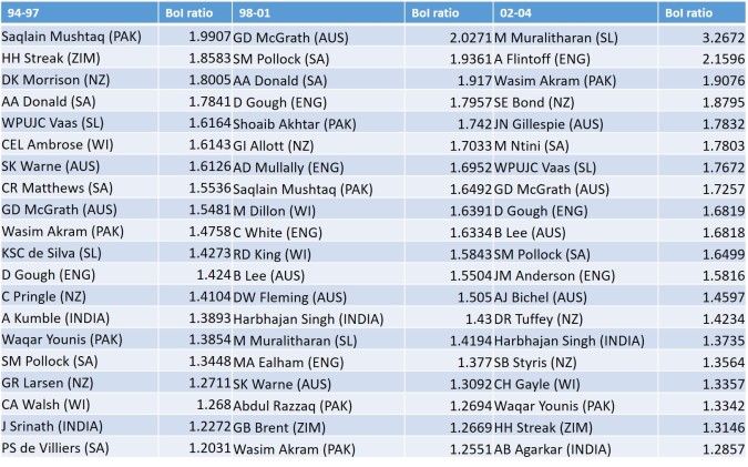
Bowlers with best BoI ratios (first innings) in the middle 3 ODI eras.
After the teams recalibrated themselves to take advantage of the powerplay, Saqlain Mushtaq bamboozled them with his many variations—the first instance of a spin bowler topping the table. The usual suspects of McGrath, Akram, Donald also make an appearance in multiple eras, but the presence of Heath Streak from a team like Zimbabwe (with no adequate support) is a significant achievement. Even in the middle 3 eras, opening bowlers have largely dominated the BoI tables barring Muralitharan and Saqlain.

Bowlers with best BoI ratios (first innings) in the last 3 ODI eras.
In the last three eras, many bowlers from the smaller teams have made it to the top rungs of the tables; this is more likely due to playing amongst themselves. This is not to diminish their achievements—they still managed to dominate their peers with the limited opportunities that were given to them. Several one day specialists have also made it to the list—Maharoof, Hafeez, Mills, Bollinger and others, showing their recent importance in the one-day format. Over the course of ODI history, many bowlers managed to breach the 2.00 mark with many hovering in its neighbourhood.
It must also be noted that the top bowlers did not maintain the same distribution across BoI values in different eras. For instance, in era 5, the top 10 are present between ~2 to ~1.6 whereas the field is much deeper in the earlier eras. Therefore, a BoI ratio cutoff of 1.40 (like in the case of batsmen) has to be applied to get a list of bowling champions. This 1.40 benchmark represents a 40% better record (in terms of BoI) with respect to the average bowler in a particular era (bowling first). But how long were these wonderful bowlers able to perform at world-beating levels?

Players having a high level of BI (1.75 or 1.40) across multiple eras.
Very few players have been able to excel the field over longer periods of time; most of them are excellent test bowlers as well. In the above table, the player’s name, and his nth appearance (in brackets) at a particular BoI ratio level has been recorded. For example, Allan Donald made his second appearance at the 1.75 level (bowling first) in the 5th ODI era. Only McGrath, Darren Gough, and Pollock have been able to maintain their dominance over three time periods; although, it must be remembered that the first era was 14 years long and Garner’s achievement has to be seen in this context. The 1.75 level has been breached in two eras only by four bowlers; the mind boggles at what Shane Bond might have achieved if not for a career cut short by injury. Several leading bowlers like Holding, Hadlee, Akram, Lee, Donald, Pollock, Kapil, Streak, Warne, Harbhajan, Steyn, and Shakib narrowly missed the 1.40 level at different points in ODI history. Overall, it has been a lot tougher for bowlers to maintain a high level of performance with respect to their peers—showing the tilt of the format towards the batsmen.
To which teams did these wonderful bowlers belong to? Did a single team have a monopoly on the world’s leading bowlers in the first innings of ODIs?

The countries with the most number of good first innings bowlers (BoI ratio>1.4) in each ODI era.
In every era, only a few bowlers have surpassed the 1.40 BoI benchmark, showing its exclusivity. In the fourth era, five teams boasted of two bowlers each from that elite list; in six other eras (Kenya wasn’t at the same level as Australia), one team had the runaway lead in terms of elite bowling arsenal. However, on-field success hasn’t necessarily followed the topmost team in the manner of batsmen in the chase, once again showing the influence of batsmen in the ODI format. Only the Australian and West Indies teams had personnel who outperformed their batting and bowling peers in the first innings. No doubt, they were the undisputed champion teams of their times, which brings us back to the 1983 World cup.
So, what were the on-field odds stacked up against the Indian team when they batted first in the 1983 World cup final?
Batting first, India had to contend with four red-hot pacemen—Roberts, Garner, Holding, and Marshall—all with first innings BoIs in excess of 1.5.l; unsurprisingly, they dislodged eight Indian batsmen that day, that too conceding only 106 runs in 42.4 overs. Undoubtedly, India’s total of 183 was low but they were also facing the most fearsome bowling attack of the time with 4 bowlers with BoI ratios greater than 1.5. Besides, West Indies were also the best chasing team at the time (with 3 top chasing batsmen in Greenidge, Richards and Lloyd). What chance did India have?
Incredibly, what followed was nothing short of a miracle. The back of the West Indian innings was broken by two dibbly-dobbly men who captured 103 wickets in 108 tests for India. And, if there was any doubt on the result being an outlier, this victory was only one of six such results in 32 matches between India and West Indies in the 1980s. No doubt, this result rankled the West Indians more than anything else. Without the shadow of a doubt, one of the greatest upsets in sporting history—which transformed the cricketing landscape—was produced on one such day when pigs sprouted wings and flew in the sky which contained a blue moon.
Disclaimer: Some images used in this article are not property of this blog. They have been used for representational purposes only. The copyright, if any, rests with the respective owners.
